Summary of Fully Convolutional Networks for Semantic Segmentation

The paper discusses “Fully Convolutional Networks for Semantic Segmentation” by Jonathan Long, Evan Shelhamer, and Trevor Darrell from UC Berkeley. The authors introduce fully convolutional networks (FCNs) as a powerful approach for semantic segmentation, surpassing existing methods in pixel-wise prediction. The key innovation is to replace fully-connected layers with convolutional layers, allowing for end-to-end training and efficient inference on arbitrary-sized inputs. The FCN architecture incorporates both deep, coarse semantic information and shallow, fine appearance information for accurate segmentations. The paper reviews related work, emphasizes the efficiency of fully convolutional training over patchwise methods, and demonstrates state-of-the-art results on various datasets. The authors compare their approach to adaptations of deep classification nets for semantic segmentation, highlighting the end-to-end learning capability of FCNs.

Fully convolutional networks Summary

In Section 3, the paper introduces fully convolutional networks (FCNs) and their key components. Each layer in a convolutional network is a 3D array, and FCNs are built on translation invariance, utilizing convolution, pooling, and activation functions. FCNs naturally operate on inputs of any size and produce corresponding spatial outputs.

The paper explains how to adapt typical classifiers for dense prediction, transforming fully connected layers into convolutional layers. This allows the network to output classification maps for inputs of any size, providing efficiency advantages.

Shift-and-stitch is introduced as a trick for dense predictions without interpolation, but the paper prefers in-network upsampling using deconvolution layers. Upsampling with factor f is described as convolution with a fractional input stride of 1/f.

Patchwise training, a form of loss sampling in stochastic optimization, is discussed. Both patchwise and fully-convolutional training can produce any distribution, but their computational efficiency depends on factors like overlap and minibatch size. The paper explores the use of sampling in patchwise training to address class imbalance and spatial correlation but finds that, in their experiments, whole image training remains effective and efficient for dense prediction.

3.1 Adapting classifiers for dense prediction

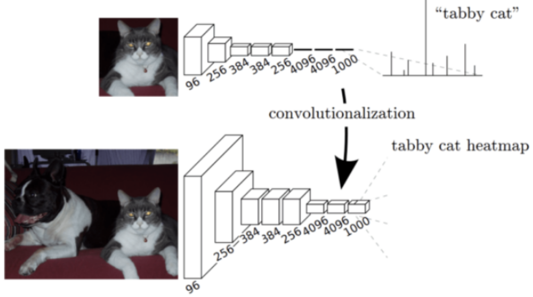
Figure 2, Transforming fully connected layers into convolution layers enables a classification net to output a heatmap.

In section 3.1, the paper discusses the adaptation of typical recognition networks, such as LeNet, AlexNet, and their successors, for dense prediction tasks. The fully connected layers in these networks, originally designed for fixed-sized inputs, can be viewed as convolutions covering their entire input regions. This transformation turns them into fully convolutional networks capable of taking inputs of any size and producing classification maps.

The illustration in Figure 2 depicts the convolutionalization process, showing how fully connected layers can output heatmaps. This adaptation allows classification nets to efficiently produce dense predictions. The computational efficiency is highlighted by comparing the processing times of the original net and its fully convolutional version.

3.2 Shift-and-stitch is filter rarefaction

In section 3.2, the paper discusses the “shift-and-stitch” technique, a method to obtain dense predictions without interpolation. It involves shifting the input for each value of (x, y) in a specific range. While it achieves denser outputs, it comes with trade-offs, including longer computation times.

3.3 Upsampling is backwards strided convolution

In section 3.3, the paper discusses the concept of upsampling in the context of connecting coarse outputs to dense pixels. Upsampling is likened to backwards strided convolution, where the fractional input stride of 1/f is achieved through convolution with a fractional output stride of f. When f is integral, upsampling can be effectively performed using backwards convolution (or deconvolution), which reverses the forward and backward passes of convolution.

3.4 Patchwise training is loss sampling

In section 3.4, the paper discusses patchwise training as a form of loss sampling in stochastic optimization. Both patchwise and fully-convolutional training can produce various distributions, with computational efficiency influenced by factors like overlap and minibatch size.

Segmentation Architecture Summary

In section 4, the paper discusses the segmentation architecture, focusing on adapting ILSVRC classifiers into FCNs for dense prediction. The authors fine-tune the networks for segmentation and introduce a novel skip architecture that combines coarse and local information to refine predictions. The experiments are conducted on the PASCAL VOC 2011 segmentation challenge, and the performance is evaluated using per-pixel multinomial logistic loss and mean pixel intersection over union.

4.1 From Classifier to Dense FCN:

The paper convolutionalizes classification architectures such as AlexNet, VGG, and GoogLeNet, converting fully connected layers into convolutions. They append a 1 × 1 convolution to predict scores for PASCAL classes and use deconvolution layers for upsampling. Results show reasonable performance after fine-tuning for segmentation.

4.2 Combining What and Where:

A new FCN for segmentation, FCN-16s, is introduced, combining predictions from different layers to enhance spatial precision. The authors experiment with a skip architecture, fusing predictions from various layers to refine the output. This fusion improves segmentation detail, and FCN-8s further incorporates predictions from lower layers.

4.3 Experimental Framework:

The optimization involves SGD with momentum, fine-tuning of all layers, and patch sampling for efficient training. The paper compares the effectiveness of whole image training versus patch sampling and finds that whole image training is as effective but converges faster. Class balancing, dense prediction through deconvolution layers, and augmentation experiments are also discussed. The models are implemented using Caffe on an NVIDIA Tesla K40c.

Results Summary

The paper evaluates the Fully Convolutional Network (FCN) on semantic segmentation and scene parsing tasks using PASCAL VOC, NYUDv2, and SIFT Flow datasets. The authors employ various metrics including pixel accuracy, mean accuracy, mean intersection over union (IU), and frequency-weighted IU.

PASCAL VOC: FCN-8s outperforms the previous state-of-the-art SDS and R-CNN on the PASCAL VOC 2011 and 2012 test sets, achieving a 20% relative improvement in mean IU. The inference time is significantly reduced compared to previous methods.

NYUDv2: Results on the NYUDv2 dataset, which includes RGB-D information, demonstrate the effectiveness of the FCN. The late fusion of RGB and HHA (depth encoding) outperforms other variations in terms of pixel accuracy, mean accuracy, mean IU, and frequency-weighted IU.

SIFT Flow: For the SIFT Flow dataset, FCN-16s achieves state-of-the-art performance on both semantic and geometric segmentation tasks. The joint model for semantic and geometric predictions performs as well as independently trained models for each task, showcasing the versatility of the FCN architecture.

Conclusion Summary

The conclusion emphasizes the significance of fully convolutional networks (FCNs) as a versatile class of models, highlighting their broader applicability beyond modern classification convolutional networks. By extending these classification networks to segmentation tasks and enhancing the architecture with multi-resolution layer combinations, the authors have achieved substantial advancements in state-of-the-art results. This improvement is not only evident in performance metrics but also in the simplification and acceleration of both learning and inference processes. The conclusion underscores the transformative impact of FCNs on various computer vision tasks, showcasing their effectiveness in addressing segmentation challenges.

Additional Knowledge

Patchwise Method

Patchwise training in computer vision involves training a model on smaller patches or sub-regions of an image rather than the entire image. Instead of feeding the entire image into the model during training, the image is divided into patches, and the model is trained on these smaller patches.

This approach has several advantages. It allows the model to focus on local features and details within an image, which can be particularly useful for tasks where local information is crucial, such as object recognition or segmentation. Patchwise training also enables the model to be more robust to variations within an image, as it learns to recognize patterns at a more granular level.

Additionally, patchwise training can help address challenges related to limited computational resources. Training on smaller patches reduces the input size, making it more feasible to train models on large datasets or high-resolution images.

Pre- and post-processing complications in the context of computer vision refer to additional steps or techniques applied before or after the main processing stages of a computer vision algorithm. Let’s break down the mentioned components:

1. Pre-processing:
   • Superpixels: Superpixels are compact and perceptually meaningful atomic regions obtained by grouping similar pixels together. They can be used as a pre-processing step to reduce the complexity of an image, making subsequent processing more efficient. Superpixels can enhance boundary information and improve segmentation results.
   • Proposals: Object proposals are candidate bounding boxes that potentially contain objects of interest. They are generated as a pre-processing step to reduce the search space for object detection tasks. Instead of exhaustively examining all possible locations, the algorithm focuses on a smaller set of proposals, improving efficiency.
2. Post-processing:
   • Random Fields: Random fields, particularly Markov Random Fields (MRFs), are used for post-hoc refinement in segmentation and classification tasks. They model spatial dependencies between pixels or regions and can improve the coherence of the final result. Random fields are often employed to enforce smoothness constraints in the output.
   • Local Classifiers: Post-hoc refinement using local classifiers involves using additional classifiers to fine-tune or correct the predictions made by the main model. This is often done at a more granular level, addressing specific regions or instances where the primary model may have made errors.

These complications are introduced to enhance the performance, robustness, and efficiency of computer vision algorithms. Superpixels and proposals help in handling complex images more effectively, while post-processing techniques like random fields and local classifiers aim to improve the precision and coherence of the final output. The goal is to address challenges such as noise, inaccuracies, or lack of global context in the initial processing stages.

The statement highlights a fundamental challenge in semantic segmentation, which is the task of assigning semantic labels to each pixel in an image. The tension referred to is between understanding the semantics (meaning or category) of objects in the image and precisely locating where these objects are.

1. Semantics vs. Location:
   • Semantics: This refers to the understanding of what objects or entities are present in the image. For example, recognizing that there are people, cars, or buildings.
   • Location: This involves determining where these objects are located in the image, the spatial information.
2. Global Information Resolves What:
   • Global information looks at the entire context of the image. Understanding the overall scene and the types of objects present falls under global information. This helps in resolving “what” is in the image at a broader level.
3. Local Information Resolves Where:
   • Local information, on the other hand, focuses on specific regions or details within the image. It helps in pinpointing “where” exactly in the image certain objects or features are located.
4. Deep Feature Hierarchies:
   • Deep feature hierarchies are a part of deep learning architectures. These hierarchies consist of layers that progressively learn more abstract and complex features. In this context, these hierarchies are jointly encoding both the location and semantics.
5. Local-to-Global Pyramid:
   • The local-to-global pyramid suggests that the model or algorithm incorporates information at different scales, ranging from local details to global context. This pyramid structure ensures that the model considers information at various levels of granularity.

In summary, the challenge in semantic segmentation is to strike a balance between understanding what is in the image (semantics) and precisely locating where these elements are situated. Deep feature hierarchies, organized in a local-to-global pyramid, are proposed to address this tension by jointly encoding both semantic and spatial information.